Linear Regression
假設模型為 y=ax+b,那麼只要兩個不同的點,就可以決定此直線了。
例如 (1,2),(4,7),那麼可以列出此聯立方程式:
{4a+b=7a+b=2
進一步寫成矩陣與向量的表示法:
[4111][ab]=[72]
Ax=b
x=A−1b
這邊可以用 [[Gaussian Elimination]], [[LU 分解]], LL 分解去解。
LSE
那如果超過兩個點呢?如果去找最適合的直線呢?
假設我們有 k 個資料點:(x1,y1),(x2,y2),…,(xk,yk),而我們要找一條直線 f(x)=ax+b,使他能最能貼近這些點的趨勢,那麼要先定義誤差:
ei=yi−f(xi)=yi−(axi+b)
這裡定義的誤差意思為,你用真實的資料點 yi 去減掉你預測出來的結果 f(xi),那就是誤差。
接著我們把他們的平方加起來(用平方而非絕對值),那麼所謂的 Loss,所謂的 Square error 則表示為:
LSE=i∑ei2=i∑(yi−f(xi))2
那我們的目標就是找到參數組合 a,b 使得誤差最小,那麼表示為:
arga,bmini∑(yi−f(xi))2
我們先展開看看:
LSE=∑i=1k(axi+b−yi)2
=[ax1+b−y1ax2+b−y2⋯]ax1+b−y1ax2+b−y2⋯
=(Ax−b)⊤(Ax−b)
=∣∣Ax−b∣∣2
其中:
Ax−b=x1x2⋮xk11⋮1k×2[ab]2×1−y1y2⋮ykk×1
∣∣Ax−b∣∣2寫成內積:
(Ax−b)1×k⊤(Ax−b)k×1
=(x⊤A⊤−b⊤)(Ax−b)
=x⊤A⊤Ax−x⊤A⊤b−b⊤Ax+b⊤b
又 x⊤A⊤b=b⊤Ax,他們都是純量,取轉置結果不變,因此:
=x⊤A⊤Ax−2x⊤A⊤b+b⊤b
接著令上面的式子為 L,又 x=[ab],來取偏微分,需要留意有 x 的項:
∂x∂L=2A⊤Ax−2A⊤b=0
那麼:
A⊤Ax=A⊤b
則:
x=(A⊤A)−1A⊤b
需要留意的是 A⊤A 是正半定矩陣(對稱),不保證可逆。
事實上,這個概念也可用投影矩陣與正交投影去理解,我們得到了參數組合 x,b 投影在 col(A) 上形成了投影向量 p(或者說是預測值 y^),而因為 p=Ax,又 x=(A⊤A)−1A⊤b,把 x 代回去,那麼得到:p=A(A⊤A)−1A⊤b,那前面這一大串作用在向量 b 的矩陣就是投影矩陣 P。
Non-Linear Regression
可以將 xi 經過函式 ϕ(x) 後得到新的特徵。
例如可以取基底 ϕ={x0,x1,x2,⋯},參見[[基底與維度#筆記 標準基底]]
舉個例子,例如取基底為 {ex,ln(x),x3}={ϕ1(x),ϕ2(x),ϕ3(x)},那麼:
y=β0+β1ϕ1(x)+β2ϕ2(x)+β3ϕ3(x)
更一般化可以如此表示,k 筆資料,基底大小為 d:
11⋮1ϕ1(x1)ϕ1(x2)⋮ϕ1(xk)⋯⋯⋱⋯ϕd(x1)ϕd(x2)⋮ϕd(xk)β0β1⋮βd
=Φβ
其中 Φ 稱為設計矩陣。
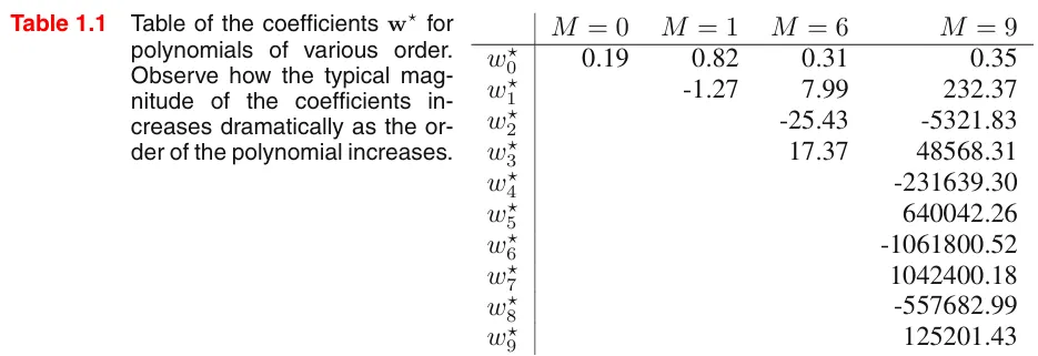
Overfitting
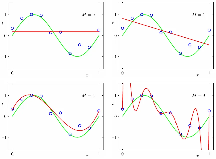
舉例來說用九次式去逼近,所有 10 個資料點都被模型的曲線給通過了,誤差為 0,每個參數取絕對值都很大,那是因為模型把噪點都學進去了,模型太複雜了。
Regularization
控制模型的參數不要那麼大(取絕對值後),那麼就把他們的值作為最小化的目標之一,因此:
argxmin(∣∣Ax−b∣∣2+λ∣∣x∣∣2)
也就是在 LSE 的基礎上,加上參數向量的長度作為「懲罰」,所謂的 L2-Norm,而調整 λ 取決於你的設定。
那麼需要最佳化的式子為:
J(x)=(Ax−b)⊤(Ax−b)+λx⊤x
展開整理,偷用之前 LSE 的結果:
接著為了後續的微分,我們把 λx⊤x 改寫成 x⊤(λI)x,以及把包含 x⊤…x 的項合併起來,整理成:
接著,為了找到讓誤差最小的極值,我們對參數向量 x 取偏微分,並令其為 0:
整理後得到:
x=(A⊤A+λI)−1A⊤b
其中,λ>0,保證 (A⊤A+λI) 是可逆的,又解決了參數的問題。
上述方法又稱為 Ridge Regularization,也就是 LSE + L2-Norm,若是用 L1-Norm,也就是 λ∣∣x∣∣1,那就是 Lasso,各有好處,因此也可以混和,例如:
LSE+λ1L1+λ2L2+⋯
Lasso 有降低維度的可能(交界在某個維度的頂點),Ridge 則讓參數權重變小。
參見L1 , L2 Regularization 到底正則化了什麼 ? | Math.py