Skip to content
The other shore
Go back

機器學習入門概念

Edit page

Linear Regression

假設模型為 y=ax+by=ax+b,那麼只要兩個不同的點,就可以決定此直線了。

例如 (1,2),(4,7)(1,2),(4,7),那麼可以列出此聯立方程式:

{4a+b=7a+b=2\begin{cases} 4a+b=7 \\ a+b=2 \end{cases}

進一步寫成矩陣與向量的表示法:

[4111][ab]=[72]\begin{bmatrix} 4 & 1 \\ 1 & 1 \end{bmatrix} \begin{bmatrix} a \\ b \end{bmatrix} = \begin{bmatrix} 7 \\ 2 \end{bmatrix} Ax⃗=b⃗\mathbf{A}\vec{x}=\vec{b} x⃗=A−1b⃗\vec{x}=\mathbf{A}^{-1}\vec{b}

這邊可以用 [[Gaussian Elimination]], [[LU 分解]], LL 分解去解。

LSE

那如果超過兩個點呢?如果去找最適合的直線呢?

假設我們有 kk 個資料點:(x1,y1),(x2,y2),…,(xk,yk)(x_1,y_1), (x_2,y_2), \dots, (x_k,y_k),而我們要找一條直線 f(x)=ax+bf(x)=ax+b,使他能最能貼近這些點的趨勢,那麼要先定義誤差:

ei=yi−f(xi)=yi−(axi+b)e_i = y_i - f(x_i)= y_i - (a x_i + b)

這裡定義的誤差意思為,你用真實的資料點 yiy_i 去減掉你預測出來的結果 f(xi)f(x_i),那就是誤差。

接著我們把他們的平方加起來(用平方而非絕對值),那麼所謂的 Loss,所謂的 Square error 則表示為:

LSE=∑iei2=∑i(yi−f(xi))2\text{LSE}=\sum_{i}{e_i}^{2}=\sum_i(y_i-f(x_i))^{2}

那我們的目標就是找到參數組合 a,ba,b 使得誤差最小,那麼表示為:

arg⁡min⁡a,b∑i(yi−f(xi))2\arg\min_{a,b} \sum_i(y_i-f(x_i))^{2}

我們先展開看看: LSE=∑i=1k(axi+b−yi)2\text{LSE} = \sum_{i=1}^k (ax_i+b-y_i)^2

=[ax1+b−y1ax2+b−y2⋯][ax1+b−y1ax2+b−y2⋯]=\begin{bmatrix} ax_1+b-y_1 & ax_2+b-y_2 & \cdots \end{bmatrix} \begin{bmatrix} ax_1+b-y_1 \\ ax_2+b-y_2 \\ \cdots \end{bmatrix}

=(Ax⃗−b⃗)⊤(Ax⃗−b⃗)= (\mathbf{A}\vec{x}-\vec{b})^{\top}(\mathbf{A}\vec{x}-\vec{b})

=∣∣Ax⃗−b⃗∣∣2= ||\mathbf{A}\vec{x}-\vec{b}||^{2} 其中:

Ax⃗−b⃗=[x11x21⋮⋮xk1]k×2[ab]2×1−[y1y2⋮yk]k×1\mathbf{A}\vec{x}-\vec{b} =\begin{bmatrix} x_1 & 1 \\ x_2 & 1\\ \vdots & \vdots \\ x_k & 1\end{bmatrix}_{k \times 2} \begin{bmatrix} a \\ b \end{bmatrix}_{2 \times 1}- \begin{bmatrix} y_1 \\ y_2 \\ \vdots \\ y_k\end{bmatrix}_{k \times 1}

∣∣Ax⃗−b⃗∣∣2||\mathbf{A}\vec{x}-\vec{b}||^{2}寫成內積:

(Ax⃗−b⃗)1×k⊤(Ax⃗−b⃗)k×1(\mathbf{A}\vec{x}-\vec{b})^{\top}_{1 \times k}(\mathbf{A}\vec{x}-\vec{b})_{k \times 1} =(x⃗⊤A⊤−b⃗⊤)(Ax⃗−b⃗)=(\vec{x}^{\top}\mathbf{A}^{\top}-\vec{b}^{\top})(\mathbf{A}\vec{x}-\vec{b}) =x⃗⊤A⊤Ax⃗−x⃗⊤A⊤b⃗−b⃗⊤Ax⃗+b⃗⊤b⃗=\vec{x}^{\top}\mathbf{A}^{\top}\mathbf{A}\vec{x}-\vec{x}^{\top}\mathbf{A}^{\top}\vec{b}-\vec{b}^{\top}\mathbf{A}\vec{x}+\vec{b}^{\top}\vec{b}

又 x⃗⊤A⊤b⃗=b⃗⊤Ax⃗\vec{x}^{\top}\mathbf{A}^{\top}\vec{b}=\vec{b}^{\top}\mathbf{A}\vec{x},他們都是純量,取轉置結果不變,因此:

=x⃗⊤A⊤Ax⃗−2x⃗⊤A⊤b⃗+b⃗⊤b⃗=\vec{x}^{\top}\mathbf{A}^{\top}\mathbf{A}\vec{x}-2\vec{x}^{\top}\mathbf{A}^{\top}\vec{b}+\vec{b}^{\top}\vec{b}

接著令上面的式子為 LL,又 x⃗=[ab]\vec{x}=\begin{bmatrix} a \\ b \end{bmatrix},來取偏微分,需要留意有 x⃗\vec{x} 的項:

∂L∂x⃗=2A⊤Ax⃗−2A⊤b⃗=0\frac{\partial L}{\partial \vec{x} }=2\mathbf{A}^{\top}\mathbf{A}\vec{x}-2\mathbf{A}^{\top}\vec{b}=0

那麼:

A⊤Ax⃗=A⊤b⃗\mathbf{A}^{\top}\mathbf{A}\vec{x}=\mathbf{A}^{\top}\vec{b}

則:

x⃗=(A⊤A)−1A⊤b⃗\vec{x}=(\mathbf{A}^{\top}\mathbf{A})^{-1}\mathbf{A}^{\top}\vec{b}

需要留意的是 A⊤A\mathbf{A}^{\top}\mathbf{A} 是正半定矩陣(對稱),不保證可逆。

事實上,這個概念也可用投影矩陣與正交投影去理解,我們得到了參數組合 x⃗\vec{x},b⃗\vec{b} 投影在 col(A)\text{col}(\mathbf{A}) 上形成了投影向量 p⃗\vec{p}(或者說是預測值 y^\hat{y}),而因為 p⃗=Ax⃗\vec{p}=\mathbf{A}\vec{x},又 x⃗=(A⊤A)−1A⊤b⃗\vec{x}=(\mathbf{A}^{\top}\mathbf{A})^{-1}\mathbf{A}^{\top}\vec{b},把 x⃗\vec{x} 代回去,那麼得到:p⃗=A(A⊤A)−1A⊤b⃗\vec{p} = \mathbf{A}(\mathbf{A}^{\top}\mathbf{A})^{-1}\mathbf{A}^{\top}\vec{b},那前面這一大串作用在向量 b⃗\vec{b} 的矩陣就是投影矩陣 PP。

Non-Linear Regression

可以將 xix_i 經過函式 ϕ(x)\phi(x) 後得到新的特徵。

例如可以取基底 ϕ={x0,x1,x2,⋯ }\phi=\{x^{0},x_1,x_2,\cdots \},參見[[基底與維度#筆記 標準基底]]

舉個例子,例如取基底為 {ex,ln⁡(x),x3}={ϕ1(x),ϕ2(x),ϕ3(x)}\{e^{x},\ln(x),x^{3}\}=\{\phi_1(x),\phi_2(x),\phi_3(x)\},那麼:

y=β0+β1ϕ1(x)+β2ϕ2(x)+β3ϕ3(x)y=\beta_0+\beta_1\phi_1(x)+\beta_2\phi_2(x)+\beta_3\phi_3(x)

更一般化可以如此表示,kk 筆資料,基底大小為 dd:

[1ϕ1(x1)⋯ϕd(x1)1ϕ1(x2)⋯ϕd(x2)⋮⋮⋱⋮1ϕ1(xk)⋯ϕd(xk)][β0β1⋮βd]\begin{bmatrix} 1 & \phi_1(x_1) & \cdots & \phi_d(x_1)\\ 1 & \phi_1(x_2) & \cdots & \phi_d(x_2)\\ \vdots & \vdots & \ddots & \vdots \\ 1 & \phi_1(x_k) & \cdots & \phi_d(x_k) \end{bmatrix} \begin{bmatrix} \beta_0 \\ \beta_1 \\ \vdots \\\beta_d \end{bmatrix} =Φβ⃗=\Phi\vec{\beta}

其中 Φ\Phi 稱為設計矩陣。

Overfitting

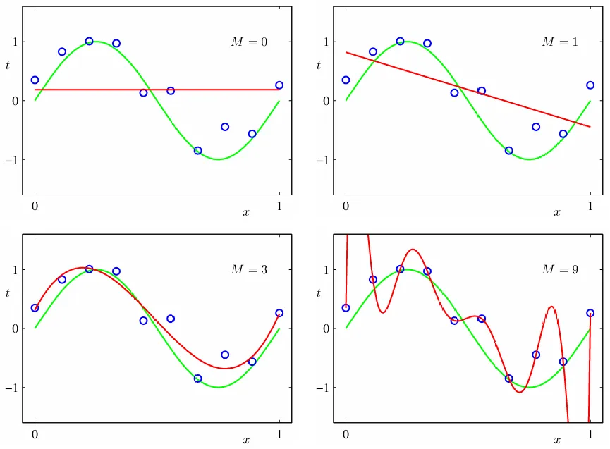
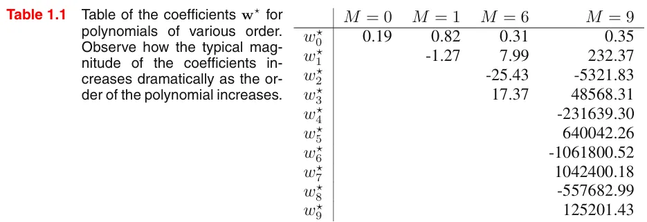
舉例來說用九次式去逼近,所有 10 個資料點都被模型的曲線給通過了,誤差為 00,每個參數取絕對值都很大,那是因為模型把噪點都學進去了,模型太複雜了。

Regularization

控制模型的參數不要那麼大(取絕對值後),那麼就把他們的值作為最小化的目標之一,因此:

arg⁡min⁡x⃗(∣∣Ax⃗−b⃗∣∣2+λ∣∣x⃗∣∣2)\arg \min_{\vec{x}} (||\mathbf{A}\vec{x}-\vec{b}||^2 + \lambda ||\vec{x}||^{2})

也就是在 LSE 的基礎上,加上參數向量的長度作為「懲罰」,所謂的 L2-Norm,而調整 λ\lambda 取決於你的設定。

那麼需要最佳化的式子為:

J(x⃗)=(Ax⃗−b⃗)⊤(Ax⃗−b⃗)+λx⃗⊤x⃗J(\vec{x})=(\mathbf{A}\vec{x}-\vec{b})^{\top}(\mathbf{A}\vec{x}-\vec{b})+\lambda \vec{x}^{\top}\vec{x}

展開整理,偷用之前 LSE 的結果:

接著為了後續的微分,我們把 λx⃗⊤x⃗\lambda\vec{x}^{\top}\vec{x} 改寫成 x⃗⊤(λI)x⃗\vec{x}^{\top}(\lambda \mathbf{I})\vec{x},以及把包含 x⃗⊤…x⃗\vec{x}^{\top} \dots \vec{x} 的項合併起來,整理成:

接著,為了找到讓誤差最小的極值,我們對參數向量 x⃗\vec{x} 取偏微分,並令其為 00:

整理後得到:

x⃗=(A⊤A+λI)−1A⊤b⃗\vec{x}=(\mathbf{A}^{\top}\mathbf{A}+\lambda \mathbf{I})^{-1}\mathbf{A}^{\top}\vec{b}

其中,λ>0\lambda \gt 0,保證 (A⊤A+λI)(\mathbf{A}^{\top}\mathbf{A}+\lambda \mathbf{I}) 是可逆的,又解決了參數的問題。

上述方法又稱為 Ridge Regularization,也就是 LSE + L2-Norm,若是用 L1-Norm,也就是 λ∣∣x⃗∣∣1\lambda||\vec{x}||_{1},那就是 Lasso,各有好處,因此也可以混和,例如:

LSE+λ1L1+λ2L2+⋯\text{LSE}+\lambda_1L_1+\lambda_2L_2+\cdots

Lasso 有降低維度的可能(交界在某個維度的頂點),Ridge 則讓參數權重變小。

參見L1 , L2 Regularization 到底正則化了什麼 ? | Math.py


Edit page
Share this post on:

Previous Post
彼岸物流第三十八章:十七歲夏天
Next Post
《異國日記》觀後感